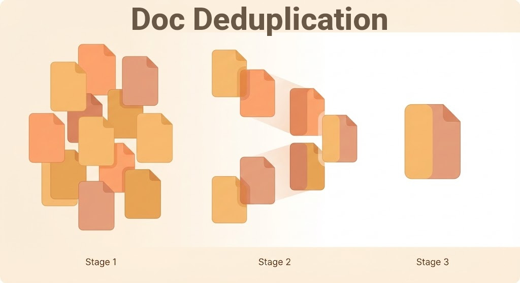
Deduplicating Documents at Scale

Deduplication sounds simple until you actually try to do it on real data.

If you have a few thousand short texts, almost any solution works. When you move to millions of long documents, multiple languages, noisy data, and the requirement to find very similar (but not identical) documents, everything changes: algorithms, data structures, memory layout, and even how you think about “similarity”.

In this post, I want to walk step by step through how deduplication evolves as scale increases:

• We’ll start with small texts and exact deduplication.
• Then move to large corpora (10+ million long documents) and the engineering challenges that appear.
• Finally, we’ll close with near‑duplicate detection: finding documents that are almost the same, but not byte‑identical.

---

1. Exact Deduplication for Small Texts

Let’s start with the simplest case: small documents (tweets, comments, short articles) and a dataset that fits comfortably in memory.

At this level, exact deduplication means: if two documents are exactly the same, keep one.

1.1 Hash‑based deduplication

The most straightforward approach is hashing the full text.

import hashlib

def hash_text(text: str) -> str:
    return hashlib.sha256(text.encode("utf-8")).hexdigest()

seen = set()
unique_docs = []

for doc in documents:
    h = hash_text(doc)
    if h not in seen:
        seen.add(h)
        unique_docs.append(doc)

Why this works:

• Hashing reduces arbitrary‑length text to a fixed‑size fingerprint.
• Set membership is O(1) on average.
• For small data, memory and CPU cost are trivial.

Please note that:

• Cryptographic hashes (SHA‑256) are overkill here.
• Collisions are theoretically possible, but practically irrelevant at this scale.

1.2 Normalization matters more than hashing

A common beginner mistake is to hash raw text.

These two documents are semantically identical, but byte‑different:

"Hello   world"
"hello world"

Before hashing, normalization is critical:

import re

def normalize(text: str) -> str:
    text = text.lower()
    text = re.sub(r"\s+", " ", text)
    return text.strip()

At small scale, normalization decisions often matter more than the dedup algorithm itself.

---

2. When Data No Longer Fits in Memory

Now let’s increase the scale.

Imagine:

• 10 million documents
• Average length: 5–20 KB
• Multiple languages
• Stored on disk or object storage

Your earlier set() approach breaks immediately.

2.1 Streaming deduplication

The first conceptual shift is streaming.

Instead of loading everything, you process documents one by one (or in batches), and store only fingerprints.

import hashlib

def hash_text(text: str) -> bytes:
    return hashlib.md5(text.encode()).digest()

Why MD5 instead of SHA‑256?

• Smaller hash (16 bytes vs 32)
• Faster
• Still perfectly fine for deduplication

At 10 million documents:

• 16 bytes × 10M ≈ 160 MB

This is already borderline, but manageable.

2.2 Disk‑backed hash sets

if the memory is not enough, don’t panic — let’s change the data structure.

Common solutions include LevelDB, LMDB or Redis.

Example using LMDB:

import lmdb
import hashlib

env = lmdb.open("dedup.lmdb", map_size=10**10)

with env.begin(write=True) as txn:
    for doc in documents:
        h = hashlib.md5(doc.encode()).digest()
        if not txn.get(h):
            txn.put(h, b"1")
            process(doc)

This pattern — hash lookup before processing — is extremely common in large pipelines.

2.3 Sorting beats hashing at massive scale

At tens or hundreds of millions of documents, even key‑value stores become expensive.

A classic large‑scale trick is:

1. Compute hashes
2. Write (hash, doc_id) to disk
3. External sort by hash
4. Remove adjacent duplicates

This works because sorting is embarrassingly parallel and disk‑friendly.

In distributed systems (Spark, Flink), this becomes almost trivial:

rdd.map(lambda d: (hash(d), d)) \
   .reduceByKey(lambda a, b: a) \
   .values()

When scale grows, algorithms that look slower on paper often win in practice.

---

3. Why Exact Deduplication Is Not Enough

So far, everything assumes exact matches but in real systems, that’s rarely enough.

Examples:

• News articles syndicated with tiny edits
• Legal documents with changed dates
• LLM‑generated content with paraphrasing

Byte‑level hashing completely fails here.

We now enter near‑duplicate detection.

---

4. From Documents to Sets: Shingling

The key idea behind near‑deduplication is this:

Compare structure instead of raw text.

4.1 k‑shingles (k-grams)

A shingle is a contiguous sequence of tokens.

from typing import List

def shingles(tokens: List[str], k: int = 5):
    return [tuple(tokens[i:i+k]) for i in range(len(tokens) - k + 1)]

Shingling converts text into a set of overlapping pieces, so that similar texts share many pieces. Here is an example:

Doc A: "data science is fun"
Doc B: "data science is awesome"
Doc C: "machine learning rocks"

word level shingles (k=2):

Doc A: ["data science", "science is", "is fun"]

Doc B: ["data science", "science is", "is awesome"]

Doc C: ["machine learning", "learning rocks"]

Two documents are similar if they share many shingles.

This naturally leads to Jaccard similarity which is:

$J(A,B)=\frac{∣A∪B∣}{∣A∩B∣}$

In our example we have this:

A = {s1, s2, s3}  # s1="data science", s2="science is", s3="is fun"
B = {s1, s2, s4}  # s4="is awesome"
C = {s5, s6}      # s5="machine learning", s6="learning rocks"

And Jaccard Index for A and B is: 2/4 = 0.5

But there’s a problem.

• A long document can have tens of thousands of shingles
• Comparing all pairs is O(n²)

This is completely infeasible at scale.

Before going forward, i like to talk more about shingles, which could be important at design level:

Choice	Impact
k (shingle size)	small k: more sensitive large k: more strict
word vs char	char-level catches typos word-level catches semantic similarity
normalization	lowercase, stemming, punctuation removal

---

5. MinHash: Compressing Similarity

MinHash is one of those algorithms that feels like magic the first time you really understand it.

Instead of storing all shingles, we store a small signature that preserves Jaccard similarity.

5.1 Conceptual intuition

• Apply multiple hash functions to each shingle
• For each hash function, keep the minimum value
• The probability that two documents share the same minimum equals their Jaccard similarity

This is the first real scaling breakthrough. Let’s learn its concept with our example. From previous section we have three sentences. Now we map them:

s1 → 1
s2 → 2
s3 → 3
s4 → 4
s5 → 5
s6 → 6

A = {1,2,3}
B = {1,2,4}
C = {5,6}

Suppose we use 2 hash functions (really simple for example):

h1(x) = (x + 1) % 6
h2(x) = (2*x + 1) % 6

Now compute min hash per document:

Doc	h1 min	h2 min
A	min(2,3,4) = 2	min(3,5,1) = 1
B	min(2,3,5) = 2	min(3,5,3) = 3
C	min(6,1) = 1	min(5,1) = 1

Now estimate Jaccard similarity for A & B:

Matching positions: 1 (h1)
Signature length: 2
Estimated Jaccard = 1/2 = 0.5

I have to mention that the Estimated value for A&C would be 0.5 but we know the real value is 0. This problem is caused because we only use two hash functions. By increasing hash functions, the estimated would accurate.

The real problem here is even with MinHash, comparing every signature pair is still O(n²). LSH comes to solve this issue.

---

6. Locality Sensitive Hashing (LSH)

MinHash gives us compact signatures.

LSH gives us candidate generation.

The idea:

• Split signatures into bands
• Hash each band
• Only compare documents that land in the same bucket

This avoids global pairwise comparison and only compare documents that have a high chance of being similar.

Let’s consider a new example where we have 3 documents with signature length of 6:

A = [2,1,3,5,4,6]
B = [2,2,3,5,1,6]
C = [6,4,2,1,3,5]

and we choose the following parameters:

• Bands = 2
• Rows per band = 3

Here are the bands:

• Band 1 = first 3 rows: [2,1,3], [2,2,3], [6,4,2]
• Band 2 = next 3 rows: [5,4,6], [5,1,6], [1,3,5]

We compute a simple hash for each band (e.g, sum mod 10):

Doc	Band 1	Band 2
A	(2+1+3)=6	(5+4+6)=15: 5
B	(2+2+3)=7	(5+1+6)=12: 2
C	(6+4+2)=12: 2	(1+3+5)=9

Band 1 buckets:

6 → A
7 → B
2 → C

Band 2 buckets:

5 → A
2 → B
9 → C

Only docs in the same bucket for any band are candidates.
Here:

• No two docs share a bucket: no candidates.
• If A & B had matched in a band: compare only that pair.

6.1 Why LSH works

LSH deliberately trades precision for speed.

• Some false positives: acceptable
• Very few false negatives: critical

In large‑scale systems, missing a duplicate is worse than checking an extra candidate.

6.2 Practical note

In production, you almost never implement LSH from scratch.

Libraries and systems:

• Datasketch (Python)
• Spark MLlib
• Custom implementations backed by Redis or Bigtable

But understanding why it works is essential when tuning thresholds.

---

7. Scaling to 10 Million Long Documents

At this scale, the problem is no longer just algorithms.

7.1 Architecture matters

A realistic pipeline looks like this:

1. Normalize text
2. Tokenize and shingle
3. Compute MinHash signatures
4. Store signatures (compressed)
5. LSH to generate candidates
6. Exact similarity check on candidates

Each step is distributed.

7.2 Storage optimization

Professionals obsess over details here:

• Store signatures as uint32
• Compress with delta encoding
• Batch writes

A signature of 128 × 4 bytes = 512 bytes

10M docs → ~5 GB

Suddenly, things are reasonable again.

---

8. Embedding-Based Deduplication: Semantic Similarity at Scale

So far, everything we discussed relies on surface-level structure: tokens, shingles, and hashing tricks.

But sometimes, you don’t care about lexical similarity at all.

You care about meaning.

Two documents can say the same thing with completely different words, structure, and length. This is where embeddings enter the picture.

---

8.1 What embeddings change conceptually

An embedding model maps a document into a dense vector in a high-dimensional space.

The promise is simple:

Documents with similar meaning end up close to each other in vector space.

Instead of asking:

• “Do these documents share many shingles?”

We now ask:

• “Are these vectors close under cosine similarity or L2 distance?”

This is a qualitative shift, not just a technical one.

---

8.2 Why embeddings are expensive

Let’s be honest: embedding-based deduplication is powerful, but costly.

Consider a realistic setup:

• 10 million documents
• 768-dimensional embeddings (very common)
• float32 values

Memory cost:

10M × 768 × 4 bytes ≈ 30 GB

This is before indexing overhead.

This is why we almost never use embeddings as the first deduplication stage.

They are usually:

• A final semantic filter
• Or applied only to already-reduced candidate sets

---

8.3 Generating document embeddings

At scale, you rarely embed raw full documents directly.

Common strategies:

• Chunk long documents
• Embed paragraphs or sections
• Aggregate (mean / max / attention-weighted)

A simple example using sentence transformers:

from sentence_transformers import SentenceTransformer
import numpy as np


model = SentenceTransformer("all-MiniLM-L6-v2")


embeddings = model.encode(
documents,
batch_size=64,
show_progress_bar=True,
normalize_embeddings=True
)

Normalization is not optional here. If you plan to use cosine similarity, normalize once and save compute forever.

---

8.4 Why naive similarity search fails

If you now try to compare every embedding to every other embedding, you’re back to O(n²).

This is not an optimization problem. This is a category error.

We need Approximate Nearest Neighbor (ANN) search.

---

9. FAISS: Similarity Search That Actually Scales

FAISS (Facebook AI Similarity Search) is the industry standard for large-scale vector similarity.

It is not magic — it is very careful engineering around:

• Vector quantization
• Memory layout
• SIMD and GPU acceleration

---

9.1 Choosing the right FAISS index

This is where most mistakes happen.

we have to choose indexes base on:

• Dataset size
• Recall requirements
• Memory budget
• Latency constraints

Some common choices:

• IndexFlatIP: exact search, zero approximation, extremely expensive
• IndexIVFFlat: inverted file, good trade-off
• IndexHNSWFlat: graph-based, very strong recall
• IndexIVFPQ: aggressive compression, lower memory

For deduplication, you almost never need exact search.

---

9.2 A practical FAISS setup

Let’s build a realistic index for deduplication.

import faiss
import numpy as np


d = embeddings.shape[1]
nlist = 4096 # number of clusters


quantizer = faiss.IndexFlatIP(d)
index = faiss.IndexIVFFlat(quantizer, d, nlist, faiss.METRIC_INNER_PRODUCT)


index.train(embeddings)
index.add(embeddings)

Key details we care about:

• Training must happen on representative data
• nlist controls recall vs speed
• Inner product + normalized vectors = cosine similarity

---

9.3 Querying for near-duplicates

Now we search for neighbors above a similarity threshold.

k = 5 # number of neighbors
D, I = index.search(embeddings, k)

Typical post-processing logic:

SIM_THRESHOLD = 0.95


near_duplicates = []


for doc_id, (scores, neighbors) in enumerate(zip(D, I)):
  for score, neighbor_id in zip(scores, neighbors):
    if neighbor_id != doc_id and score >= SIM_THRESHOLD:
      near_duplicates.append((doc_id, neighbor_id, score))

This gives you semantic near-duplicates — not just lexical ones.

---

9.4 When embeddings are the wrong tool

It’s important to say this explicitly.

Embeddings are not ideal when:

• You need strict guarantees
• Documents differ only in boilerplate
• You must explain why two docs are duplicates

They shine when:

• Paraphrasing exists
• Language varies
• Structure is unreliable

10. Final Thoughts: Duplicate Hunting

Deduplication is not a single algorithm.

It’s a progressive refinement process:

• Start cheap
• Eliminate obvious duplicates early
• Spend CPU only where it matters

Exact deduplication removes noise.
Near‑duplicate detection removes redundancy.

At scale, the real skill is not knowing MinHash or LSH — it’s knowing where in the pipeline to apply them, and how much accuracy you can afford to lose.

If there’s one takeaway, it’s this:

Good deduplication systems are engineered, not just implemented.

And once you’ve built one, you’ll never look at “remove duplicates” the same way again.